domingo, 9 de dezembro de 2018

Deep Learning wih PyTorch


Deep Learning wih PyTorch

Using MNIST Datasets

PyTorch is an open-source machine learning library for Python, based on Torch, used for applications such as natural language processing. It is primarily developed by Facebook's artificial-intelligence research group, and Uber's "Pyro" software for probabilistic programming is built on it.
The MNIST dataset
The MNIST dataset was constructed from two datasets of the US National Institute of Standards and Technology (NIST). The training set consists of handwritten digits from 250 different people, 50 percent high school students, and 50 percent employees from the Census Bureau. Note that the test set contains handwritten digits from different people following the same split.
The MNIST dataset is publicly available at http://yann.lecun.com/exdb/mnist/ and consists of the following four parts:
- Training set images: train-images-idx3-ubyte.gz (9.9 MB, 47 MB unzipped, and 60,000 samples)
- Training set labels: train-labels-idx1-ubyte.gz (29 KB, 60 KB unzipped, and 60,000 labels)
- Test set images: t10k-images-idx3-ubyte.gz (1.6 MB, 7.8 MB, unzipped and 10,000 samples)
- Test set labels: t10k-labels-idx1-ubyte.gz (5 KB, 10 KB unzipped, and 10,000 labels)
PyTorch provides two high-level features:
a) Tensor computation (like NumPy) with strong GPU acceleration
b) Deep Neural Networks built on a tape-based autodiff system
To keep things short:
PyTorch consists of 4 main packages:
torch: a general purpose array library similar to Numpy that can do computations on GPU when the tensor type is cast to (torch.cuda.TensorFloat)
torch.autograd: a package for building a computational graph and automatically obtaining gradients
torch.nn: a neural net library with common layers and cost functions
torch.optim: an optimization package with common optimization algorithms like SGD,Adam, etc

PyTorch Tensors

In terms of programming, Tensors can simply be considered multidimensional arrays. Tensors in PyTorch are similar to NumPy arrays, with the addition being that Tensors can also be used on a GPU that supports CUDA. PyTorch supports various types of Tensors.

Look for development details on my GitHub.

References:

My GitHub: 

sábado, 8 de dezembro de 2018

History of the Web


Sir Tim Berners-Lee is a British computer scientist. He was born in London, and his parents were early computer scientists, working on one of the earliest computers.
Growing up, Sir Tim was interested in trains and had a model railway in his bedroom. He recalls:
“I made some electronic gadgets to control the trains. Then I ended up getting more interested in electronics than trains. Later on, when I was in college I made a computeout of an old television set.”
After graduating from Oxford University, Berners-Lee became a software engineer at CERN, the large particle physics laboratory near Geneva, Switzerland. Scientists come from all over the world to use its accelerators, but Sir Tim noticed that they were having difficulty sharing information.
“In those days, there was different information on different computers, but you had to log on to different computers to get at it. Also, sometimes you had to learn a different program on each computer. Often it was just easier to go and ask people when they were having coffee…”, Tim says.
Tim thought he saw a way to solve this problem – one that he could see could also have much broader applications. Already, millions of computers were being connected together through the fast-developing internet and Berners-Lee realised they could share information by exploiting an emerging technology called hypertext.
In March 1989, Tim laid out his vision for what would become the web in a document called “Information Management: A Proposal”. Believe it or not, Tim’s initial proposal was not immediately accepted. In fact, his boss at the time, Mike Sendall, noted the words “Vague but exciting” on the cover. The web was never an official CERN project, but Mike managed to give Tim time to work on it in September 1990. He began work using aNeXT computer, one of Steve Jobs’ early products.

https://webfoundation.org/about/vision/history-of-the-web/

segunda-feira, 3 de dezembro de 2018

Worldwide Steel Production with Machine Learning


The objective of this work is to analyze the production of iron and steel using machine learning. The data was obtained from web sites of the specialty and gives a greater emphasis to the production in South America and Brazil in particular.
The information was collected on the websites:
The information about year 2018, is real information from January to October 2018 and is projected to November and December 2018, because we are ending November 2018.
This work also trains the use of interactive maps of the folium package, to present the statistics. I used the Collaborative Jupyter Notebook, from Google, to made this work. Complete python work is in Github.
The data sources to create graphs are in Github (folder data) in excel format.
Let’s go work.
Because I am in collaborative jupyter, I read the files to the platform with code:


Need install package xlrd to read excel files.


Files to read:


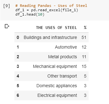
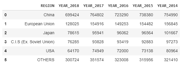
Some read tables from excel:


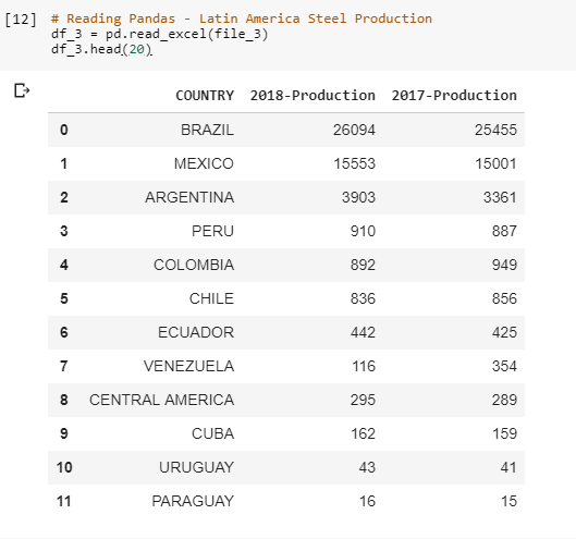
Table with Latin America production:


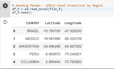
I created a file with geo-coordinates from latin america countries, to plot stats in a map:


Printing Graphs:


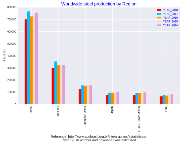
Steel Production By Region


The graph shows a decline in iron and steel production in 2018 in all markets.
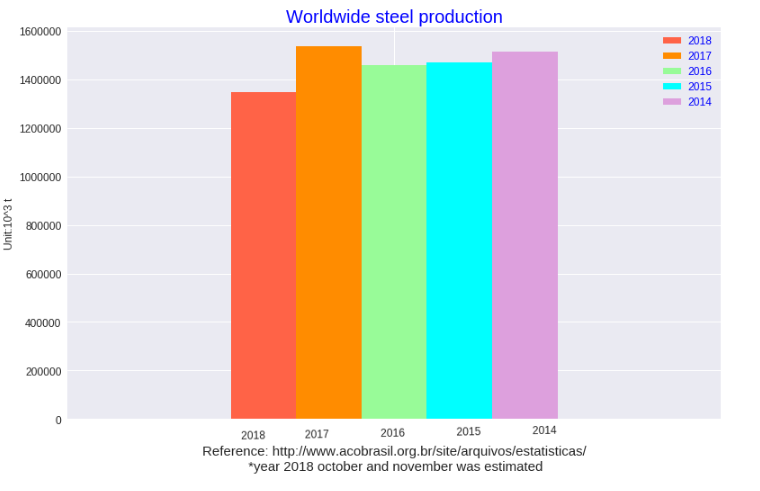
Making a Sum of all markets:


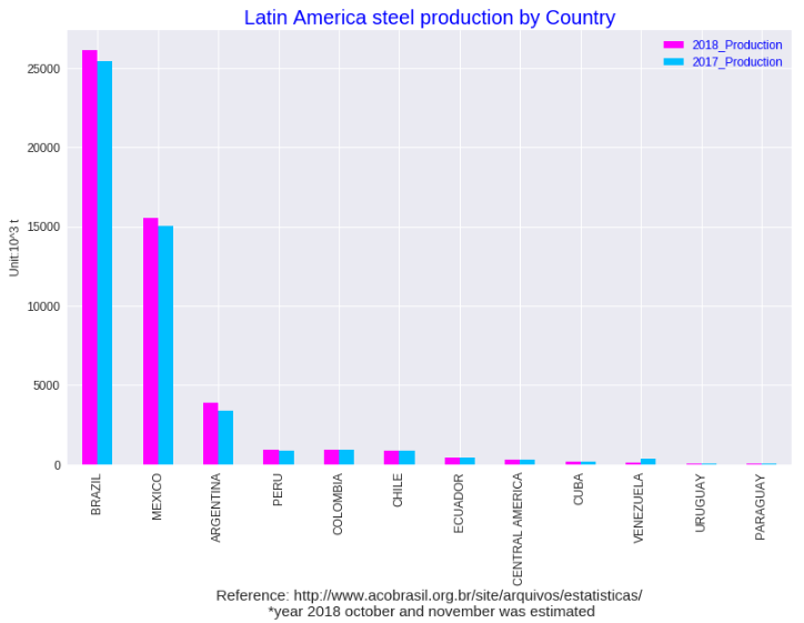
Latin America Production


Creating Maps with Folium package

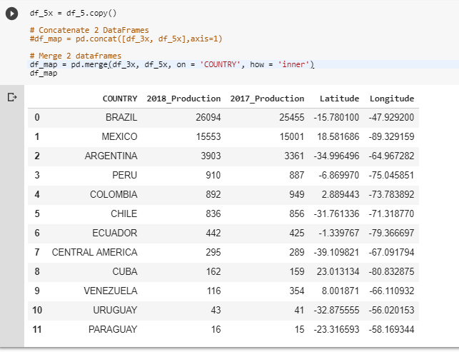
I made a merge with the Latin America table with the table with geographic data:


We need install folium package, to create interactive maps:


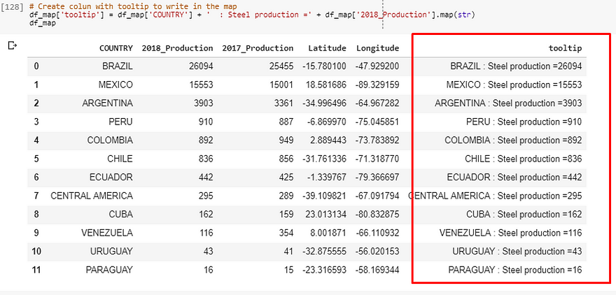
I create a new column in the dataframe to make the tootip that i want to present un the flag-mark.


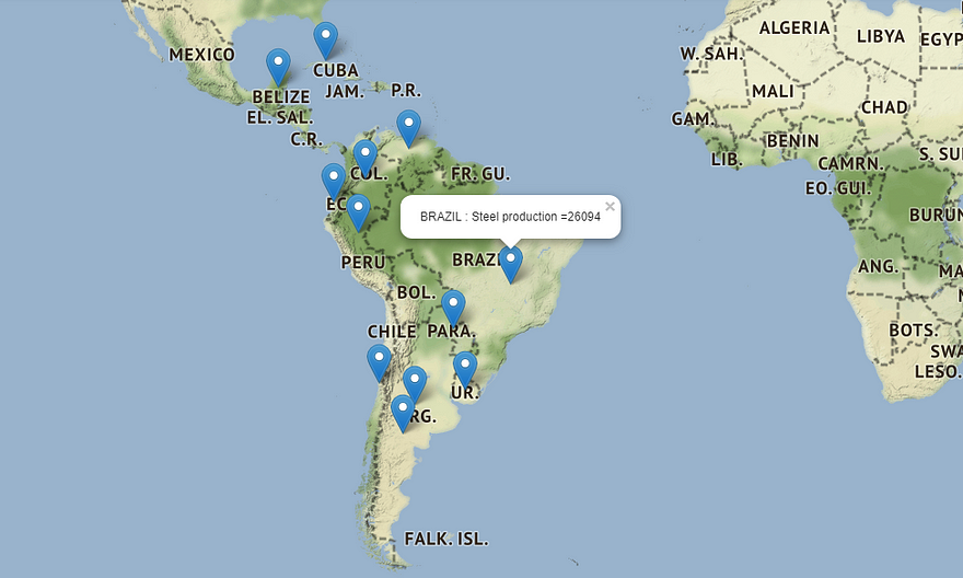
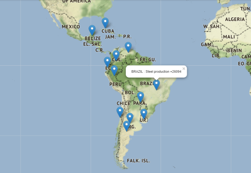
To print the stats in the map, I used the code bellow. I used the dataframe to pass the coordinates to the map.


The system creates a beautiful map. When we click in the mark-flag the system presents the name of the country and it’s steel production.

Steel Products from Brazil

Because i’m in Brazil, let’s go watch what’s up here.


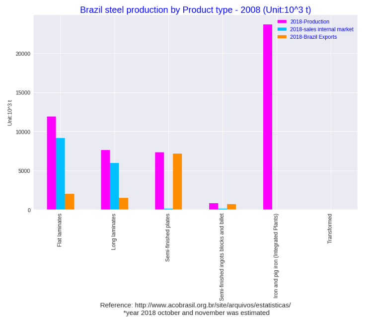
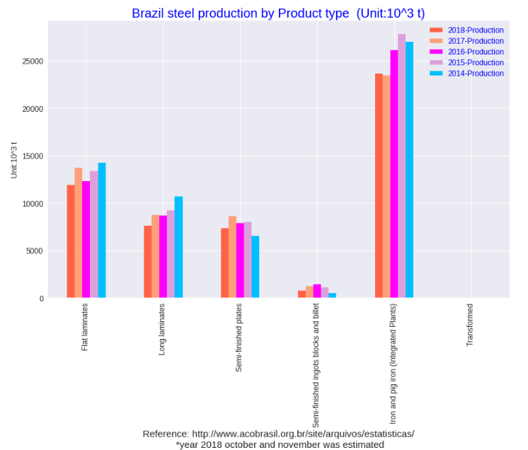
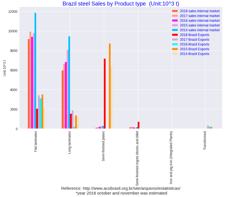
I have many informations by year, about production and sales. I make separate graphs to explore the information.


Creating subsets dataframes to make prints, in that case about production by year:


In this chart we see the same trend, that production in 2018 is lower than in 2017, in all types of steel products.
Creating a subset dataframe with Brazil Steel Sales:


Sales in 2018 are lower than in 2017, both in the domestic market and in exports.

Conclusion:

At the conclusion of this work, there is the knowledge about the steel and iron production market, the best knowledge in the Brazilian market. Printing on an interactive geographic map will be an excellent tool for presenting future work on websites.
Original article on Medium:
https://medium.com/datadriveninvestor/worldwide-steel-production-with-machine-learning-7796b423e2ea

Placing statistics on geographic maps can be simple


Testing some functionality from package folium to making interactive geographic graphs with statistical information, I found the APP datawrapper, which can make it easy and that in a moment of having to be practical and efficient to make a presentation … may be the solution.
The datawrapper APP creates interactive graphs including your stats information. You have a screen to input you data by country, by region, or you can import your csv table.
You can configure your title, your labels, put your source information, configure colors, and insert tooltip information when the mouse its in the country.
Because I’m studying about steel, I have some statistical information about world steel production in 2018, obtained here and in that web page.
According to information from the company that manages the wep page consulted, the data was obtained based on actual production data until October 2018 and projecting November and December 2018.

Plotting the information in a Geographic map


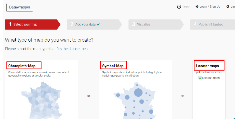
  1. 1.Select map type on https://app.datawrapper.de

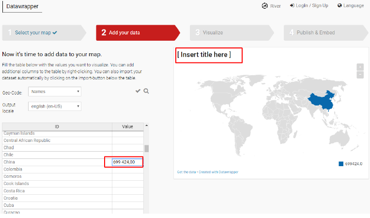
2. Write your data in the left table


3. Configure your title, color and notes


4. Customize your tootlip information


5. Customize your legends


6. Publish your map


You obtain an link or an embed code, to put in your website.
Conclusion:
Easy, very easy. Beautiful and useful APP. Look here…